ConvNext
This paper is best described in its abstract as ‘We gradually “modernize” a standard ResNet toward the design of a vision Transformer, and discover several key components that contribute to the performance difference along the way’.
What we’ll try to learn through building ConvNext is the meaning behind these design choices in terms of:
- Activation Functions
- Architechture
- Inductive Biases
- And more so ..
Why I Love ConvNext
This is one of the few architechtures which I have re-written from scratch including the Dataloaders. I used ConvNext for Face Classification and beat 250+ students and TAs in my class on a Kaggle Competition.
I not only re-wrote it in a simple manner, I also had to make many design decisions in reducing the channel widths and reducing network depth to brind down the trainable params from 29 Million to just 11 million

Table of contents
Introduction
Drawbacks of Vanilla Vision Transformers (ViTs)
- ViTs became famous due to their ability to scale
- With huge datasets they outperformed ResNets on Image Classification
- However, ironically, the cost of global attention (to all tokens i.e. all image patches fed to the transformer) grows quadratically with image size
- For real world images, this issue is a big problem!
Enter Hierarchial ViTs like SWIN Transformer
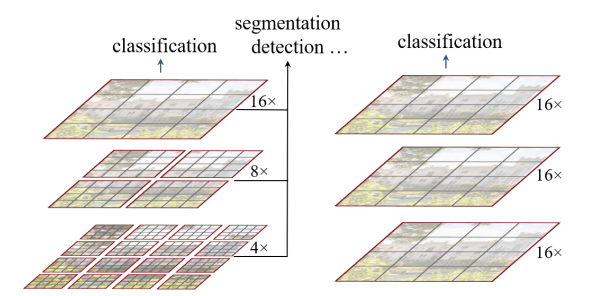
- Instead of just global attention, introduce attention locally to a window (red boundary)
- A fixed number of image patches form a window
-
This reduces the time complexity from being quadratic in image size for generic ViTs to now being linear w.r.t image size
- This linear time complexity w.r.t image size made ViTs tractable for all vision tasks like detection, segmentation and classification
Approach
The use of shifted-windows as in Swin Transformers and the learnings from the era of ViTs motivate the authors of ConvNext to begin ‘modernizing’ CNNs.
They begin by taking a simple ResNet-50 model and reshaping it from the learning of ViTs. They do this in two steps:
- New Training Methods
- New Network Architectures which include:
- Macro Design changes
- ResNextify
- Inverted Bottleneck
- Larger Kernel Sizes
- Layer-wise micro designs
Training Optimizations
This mainly included new optimizers, larger training epochs, and new augmentation methods. Specifically:
- AdamW over Adam
- Augmentations such as: Mixup, Cutmix, RandAugment, Random Erasing
- Regularization schemes including Stochastic Depth and Label Smoothing
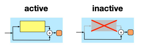
Stochastic depth is when we choose to keep a residual block active or inactive based on some probability (maybe bernoulli or a uniform probability distribution) as shown below:
Network Modernization
Understanding ResNets
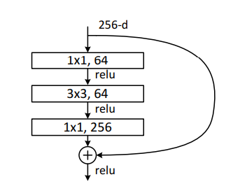
It’s beneficial to first see how a resnet works. Firstly note that we have two variants of the ResNet block
- Simple Block (used in ResNet34)
- BottleNeck Block (used in all other ResNets)
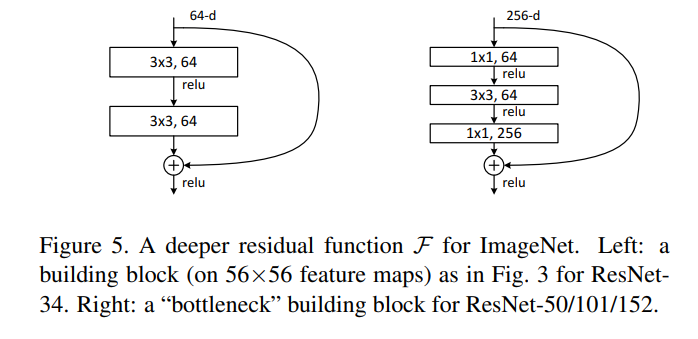
The overall architechture of Resnet is captured in the below diagrams:
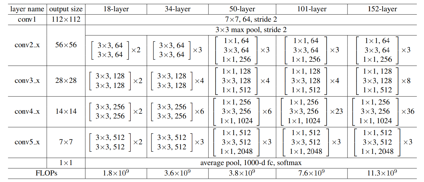
Where the final 1000x1 vector is for the 1000 ImageNet classes. Also note the number of repeating ResNet block in each layer (50-layer or ResNet50 being referred below):
- Conv2_x has 3 blocks
- Conv3_x has 4 blocks
Overall we have (3,4,6,3) as ‘stage compute ratio’ as defined by authors.
Macro Design
We saw (3,4,6,3) as ‘stage compute ratio’ in ResNet50 as explained previously. In Swin-Transformer the same block distribution was (1,1,9,1).
Hence, ConvNext tries to follow the same and uses (3,3,9,3) as the block distributions.
Making it more Lean (to reduce params)
However, I had to cut down on this to reduce parameter limit and changed the ratios to (6,5,4,4). This was chosen after a few ablations but also higher numbers for the initial blocks were chosen to allow for an optimization on the number of channels at input/output of each ConvNext stage. Specifically:
# number of channels at input/output of each res_blocks
# Updated Config
self.channel_list = [50, 175, 250, 400]

# Original Config
# self.channel_list = [96, 192, 384, 768]

# number of repeats for each res_block
# Updated Config
self.block_repeat_list = [6,5,4,4]

# Original Config
# self.block_repeat_list = [3,3,9,3]
As you can see, to maintain the relative number of channels at each stage (at least keep it monotonically increasing as in the original config), I had to increase the initial block_repeats where the channel size is small and decrease the block_repeats when channel size was larger
ResNextify
ResNext utilized group convolution in the 3x3 conv layer of bottleneck blocks. What is group convolution?
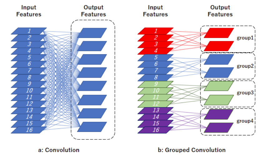
The authors of ConvNext decided to use a special case of group convolution where the number of groups equals number of channels. That is literally just Depthwise Seperable Convs!!!
Why Depthwise Convolutions
Depthwise Seperable Conv has two stages: Depthwise Conv (KxKx1 filters) & Pointwise Conv (1x1xC filters)
The simple answer is the computational complexitites:
- Depth-wise Separable =
O(n**2*d + n*d**2)-> as per Attention is all you need - Generic Convolution =
O(n**2 * d**2)-> Think of n = filter size spatial, d = filter size depth (num channels) - Reference : MobileNet
- Reference : Attention is All You Need
However, while those numbers may seem weird, for a more practical example you can view this post.
Bottomline, MobileNet shows that Depthwise Seperable Conv has much lesser FLOPs than conventional convolution layers.
There is also some super cool intuition on how Depthwise + Pointwise Conv is similar to Self Attention!
We note that depthwise convolution is similar to the weighted sum operation in self-attention, which operates on a per-channel basis, i.e., only mixing information in the spatial dimension.
That’s a little painful to understand. But first read this nice blog to understand the process of self-attention.
In that blog, we have a values matrix had shape values.shape: torch.Size([6, 28]). We then compute the attention weights for the second word (second token).
NOTE: Computing attention_weights for second token means using q_2 matrix and multiplying it with k_1, k_2, k_3, k_4, k_5, k_6 and then some softmax. But intuition is that second word was the query or our anchor and we wanted to see how all other words are close/far from second word.
So, if second word is our query, and we got attention weights attention_weights_2, which has shape 1x6. We then multiply this attention_weights_2 with the values matrix which comprises ALL words/tokens and has shape 6x28
So finally, the attention_weights_2 @ values yields a 28x1 size context vector which is just one output of the self-attention head.
But, the intuition of Depthwise seperable convolution that comes here is that:
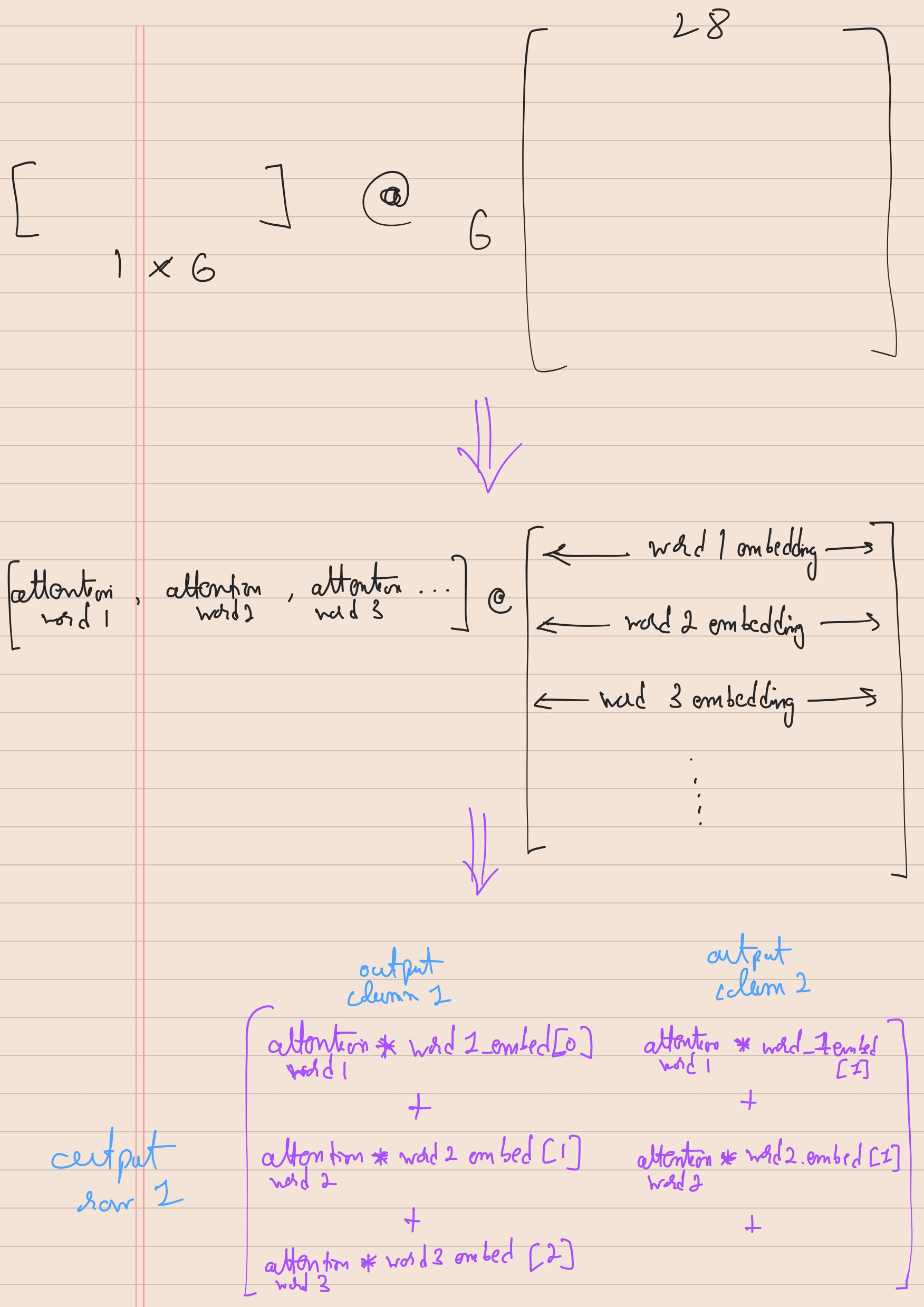
In the above picture, we see that attention of word_1 get’s multiplied with word 1’s positional embedding and there is no cross over. That’s the best understanding I could infer from the statement.
Inverted BottleNeck and Large Kernels
Inverted bottlenecks were made famous long back by MobileNetV2 and that design stuck even with Transformers
| ResNet Bottleneck | Proposed ConvNext Bottleneck |
|---|---|
 | 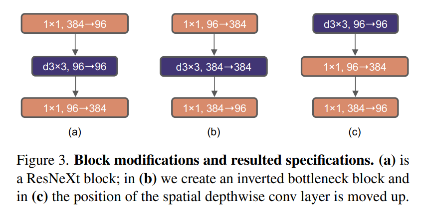 |
Another aspect to note is that depthwise conv was moved up. The reasoning for this is as follows:
- We want to emulate the Swin-T’s large kernel size. We only have one spatial conv layer (that too is depthwise (
d3x3)) - If we do
d3x3as in the middle design of ConvNext Bottleneck that’ll bed3x3with 384 channels - Instead if we move it up earlier, the spatial
d3x3Conv happens with 96 channels, similarly the pointwise 1x1 conv happens across 384 channels - So the 1x1 does the heavy lifting but it’s fast, the
d3x3satisfies the large kernel size requirement with low number of channels
To push this further, we increase d3x3 to d7x7 to exactly match the Swin Transformer:
Activations
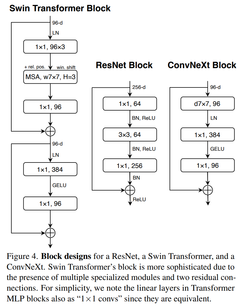
This was very well written in the ConvNext paper, I’m directly quoting it here: Consider a Transformer block with key/query/value linear embedding layers, the projection layer, and two linear layers in an MLP block. There is only one activation function present in the MLP block. In comparison, it is common practice to append an activation function to each convolutional layer, including the 1 × 1 convs. Here we examine how performance changes when we stick to the same strategy. As depicted in Figure 4, we eliminate all GELU layers from the residual block except for one between two 1 × 1 layers, replicating the style of a Transformer block. This process improves the result by 0.7% to 81.3%, practically matching the performance of Swin-T.
So we essentially:
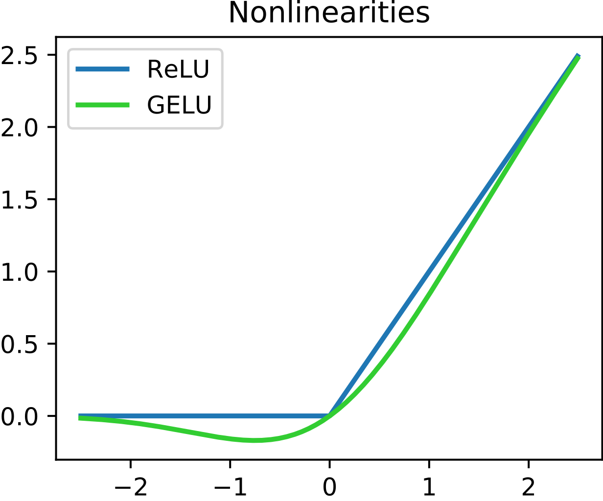
- Replaced ReLU with GELU
- Reduced the number of activations
- They also reduced the number of normalizations (mentioned later)
Implementation
ConvNext Block
class ConvNextBlock(torch.nn.Module):
    """
    Refer : https://browse.arxiv.org/pdf/2201.03545v2.pdf for detailed architechture

    """

    def __init__(self, num_ch, expansion_factor, drop_prob=0.0):
        # num_ch = number of channels at first and third layer of block
        # There'll be an expansion in the second layer given by expansion_factor
        super().__init__()

        """
        NOTE: To perform depthwise conv we use the param (groups=num_ch)
        to create a separate filter for each input channel
        """


        self.main_block = torch.nn.Sequential(
            # 1st conv layer (deptwise)
            torch.nn.Conv2d(in_channels=num_ch, out_channels=num_ch,
                            kernel_size=7, padding=3, groups=num_ch),
            torch.nn.BatchNorm2d(num_ch),

            # 2nd conv layer
            torch.nn.Conv2d(in_channels=num_ch, out_channels=num_ch*expansion_factor, kernel_size=1, stride=1), # 1x1 pointwise convs implemented as Linear Layer
            torch.nn.GELU(),

            # 3rd conv layer
            torch.nn.Conv2d(in_channels=num_ch*expansion_factor, out_channels=num_ch, kernel_size=1, stride=1)
        )

        for layer in self.main_block:
            if isinstance(layer, torch.nn.Conv2d):
                init.trunc_normal_(layer.weight, mean=config['truncated_normal_mean'], std=config['truncated_normal_std'])
                init.constant_(layer.bias, 0)

        # define the drop_path layer
        if drop_prob > 0.0:
            self.drop_residual_path = DropPath(drop_prob)
        else:
            self.drop_residual_path = torch.nn.Identity()

    def forward(self, x):
        input = x.clone()
        x = self.main_block(x)

        # sum the main and shortcut connection
        x = input + self.drop_residual_path(x)

        return x
Network Setup
class Network(torch.nn.Module):
    """
    ConvNext
    """

    def __init__(self, num_classes=7001, drop_rate=0.5, expand_factor=4):
        super().__init__()

        self.backbone_out_channels = 400
        self.num_classes = num_classes

        # number of channels at input/output of each res_blocks
        self.channel_list = [50, 175, 250, 400]
        # self.channel_list = [96, 192, 384, 768]

        # number of repeats for each res_block
        self.block_repeat_list = [6,5,4,4]
        # self.block_repeat_list = [3,3,9,3]

        # define number of stages from above
        self.num_stages = len(self.block_repeat_list)

        self.drop_path_probabilities = [i.item() for i in torch.linspace(0, drop_rate, sum(self.channel_list))]

        ############## DEFINE RES BLOCK AND AUX LAYERS ########################

        # # Define the Stem (the first layer which takes input images)
        self.stem = torch.nn.Sequential(
            torch.nn.Conv2d(in_channels=3, out_channels=self.channel_list[0], kernel_size=4, stride=4),
            torch.nn.BatchNorm2d(self.channel_list[0]),
            )

        # truncated normal initialization
        for layer in self.stem:
            if isinstance(layer, torch.nn.Conv2d):
                init.trunc_normal_(layer.weight, mean=config['truncated_normal_mean'], std=config['truncated_normal_std'])
                init.constant_(layer.bias, 0)

        # # Store the LayerNorm and Downsampling layer when switching btw 2 types of res_blocks
        # self.block_to_block_ln_and_downsample = []
        self.block_to_block_ln_and_downsample = [self.stem]
        for i in range(self.num_stages - 1):
            inter_downsample = torch.nn.Sequential(
                    torch.nn.BatchNorm2d(self.channel_list[i]),
                    torch.nn.Conv2d(in_channels=self.channel_list[i],
                                    out_channels=self.channel_list[i+1],
                                    kernel_size=2, stride=2)
                  )
            self.block_to_block_ln_and_downsample.append(inter_downsample)

        # Store the Res_block stages (eg. 3xres_2, 3xres_3, ...)
        self.res_block_stages = torch.nn.ModuleList()
        for i in range(self.num_stages):
            res_block_layer = []
            for j in range(self.block_repeat_list[i]):
                res_block_layer.append(ConvNextBlock(num_ch=self.channel_list[i],
                                  expansion_factor=expand_factor,
                                  drop_prob=self.drop_path_probabilities[i+j]))

            # append the repeated res_blocks as one layer
            # *res_block_layer means we add individual elements of the res_block_layer list
            self.res_block_stages.append(torch.nn.Sequential(*res_block_layer))

        # truncated normal initialization
        for res_block_stage in self.res_block_stages:
            for layer in res_block_stage:
                if isinstance(layer, torch.nn.Conv2d):
                    init.trunc_normal_(layer.weight, mean=config['truncated_normal_mean'], std=config['truncated_normal_std'])
                    init.constant_(layer.bias, 0)

        #####################################################################

        self.backbone = torch.nn.Sequential(
              # essentially stem (replace with stem if it works)
              self.block_to_block_ln_and_downsample[0],
              # res_1 block
              self.res_block_stages[0],
              self.block_to_block_ln_and_downsample[1],
              # res_2 block
              self.res_block_stages[1],
              self.block_to_block_ln_and_downsample[2],
              # res_3 block
              self.res_block_stages[2],
              self.block_to_block_ln_and_downsample[3],
              # res_4 block
              self.res_block_stages[3],
              torch.nn.AdaptiveAvgPool2d((1,1)),
              torch.nn.Flatten(),
            )

        self.cls_layer = torch.nn.Sequential(
            torch.nn.Linear(self.backbone_out_channels, self.num_classes))

        # truncated normal initialization
        for layer in self.cls_layer:
            if isinstance(layer, torch.nn.Linear):
                init.trunc_normal_(layer.weight, mean=config['truncated_normal_mean'], std=config['truncated_normal_std'])
                init.constant_(layer.bias, 0)

    def forward(self, x, return_feats=False):
        """
        What is return_feats? It essentially returns the second-to-last-layer
        features of a given image. It's a "feature encoding" of the input image,
        and you can use it for the verification task. You would use the outputs
        of the final classification layer for the classification task.
        """
        feats = self.backbone(x)
        out = self.cls_layer(feats)

        if return_feats:
            return feats
        else:
            return out

model = Network().to(DEVICE)
summary(model, (3, 224, 224))
Stochastic Depth and Training
class DropPath(torch.nn.Module):
    """
    Stochastic Depth (we drop the non-shortcut path inside residual blocks with
                      some probability p)
    """

    def __init__(self, drop_probability = 0.0):
        super().__init__()
        self.drop_prob = drop_probability

    def forward(self, x):
        # if drop prob is zero or in inference mode, skip this
        if np.isclose(self.drop_prob, 0.0, atol=1e-9) or not self.training:
          return x

        # find output shape (eg. if input = 4D tensor, output = (1,1,1,1))
        # output_shape = (x.shape[0],) + (1,) * (x.ndim - 1)
        output_shape = (x.shape[0],1,1,1)

        # create mask of output shape and of input type on same device
        keep_mask = torch.empty(output_shape, dtype=x.dtype, device=DEVICE).bernoulli_((1-self.drop_prob))
        # Alternative: random_tensor = x.new_empty(shape).bernoulli_(keep_prob)

        # NOTE: all methods like bernoulli_ with the underscore suffix means they
        # are inplace operations
        keep_mask.div_((1-self.drop_prob))

        return x*keep_mask

criterion = torch.nn.CrossEntropyLoss(label_smoothing=0.1) # multi class classification, hence CELoss and not BCELoss
optimizer = torch.optim.AdamW(model.parameters(), lr=config['lr'], betas=(0.9, 0.999), weight_decay=0.05)

gamma = 0.6
milestones = [10,20,40,60,80]

# scheduler1 = torch.optim.lr_scheduler.ConstantLR(optimizer, factor=0.9, total_iters=5)
scheduler = torch.optim.lr_scheduler.MultiStepLR(optimizer, milestones=milestones, gamma=gamma)
# scheduler3 = torch.optim.lr_scheduler.ReduceLROnPlateau(optimizer, 'min')
# scheduler = torch.optim.lr_scheduler.SequentialLR(optimizer, schedulers=[scheduler1, scheduler2, scheduler3], milestones=[20, 51])

scaler = torch.cuda.amp.GradScaler()
Appendix
Time Complexities Analyses
Simple Matrix Multiplication
In general if we are multiplying two matrices A (of size {N,D}) and B (of size {D,D}) then A@B will involve three nested loops, specifically:
- For each of the N rows in A
- We perform D dot products
- Which each involves D multiplictions
- We perform D dot products
Hence, overall time complexity = N * D * D = N * D**2
Time Complexity Analysis in Tranformers
The transformers are seq2seq models with desired output (during training) is just the right shifted inputs. For example if input is ‘I am superman’ and we are building a word2word prediciton language model given input I the desired output is am and that makes:
- OurInput =
<SOS> I am Superman - Desired output =
I am Superman <EOS>
Consider we have N words which we project in embedding layer where each word gets projected to a vector of shape D, then a sentence of N words will get projected to a shape of N x D (just a matrix where num_rows = num_words and num_cols = projection_size)
Then self attention in scaled-dot-product form:
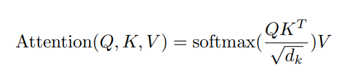
Will have the following time comlexity
- Linearly transforming the rows of
Xto compute the queryQ, keyK, and valueVmatrices, each of which has shape(N, D). This is accomplished by post-multiplyingXwith 3 learned matrices of shape(D, D), amounting to a computational complexity ofO(N D^2). - Computing the layer output, specified in above equation of the paper as
SoftMax(Q @ Kt / sqrt(d)) V, where the softmax is computed over each row. ComputingQ @ Kthas complexityO(N^2 D), and post-multiplying the resultant withVhas complexityO(N^2 D)as well.
Overall the time complexity would be O(N^2.D + N.D^2)
NOTE: In the paper, they say it takes only O(N^2 D) for Self Attention, but this excludes the calculation of Q,K,V
Comparison with RNNs
RNNs have a hidden state neuron which is connected across the time series as shown below:
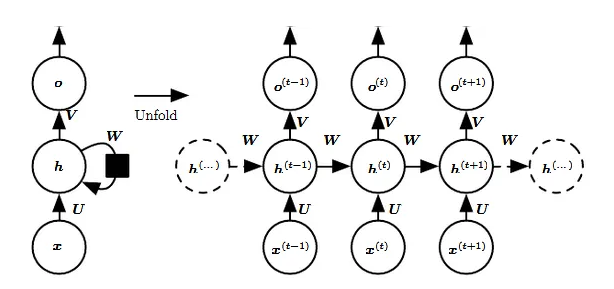
The hidden neuron computation is simply: h(t) = f(U x(t) + W h(t−1))
Hence, they are modelled as O(n * d*2) *(as it’s an MLP with matrix multiplication, see Appendix) with O(n) sequential operations
Comparisons with Separable and Non-Separable Convs
- Depth-wise Separable =
O(n**2*d + n*d**2)= Self Attention + Feed Forward MLP - Generic Convolution =
O(n**2 * d**2)
Conclusion:
The authors of Attention is All You Need therefore claim that Self Attention (O(N**2*D) or truly O(N**2*D + N*D**2)) is parallelizable and faster than the next best option -> i.e. Depthwise Separable Convolution (O(N**2*D + N*D**2))
Considering the true calculation of Scaled Dot Product Attention, it seems to be the same as Depthwise Separable Convolution.