Table of contents
Before you Begin
Reference Book 1 Reference Book 2
PDFs
Some Basics on Camera Projection
Projection of 3D to 2D image plane
To understand how a camera views the 3D world, first we look at the projection of 3D points onto an image plane. We use basic high school physics and some similar triangle properties to derive the following formula:
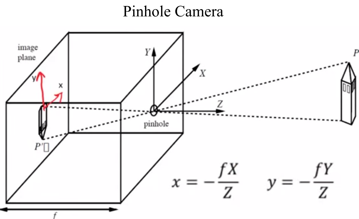
Notice that the minus sign is bit irritating to work with. (Also we don’t see inverted images as the formula suggests. This is becauase our brain does the inversion in real time)
Therefore, let’s start with the below version of the formula by ignoring this inversion effect
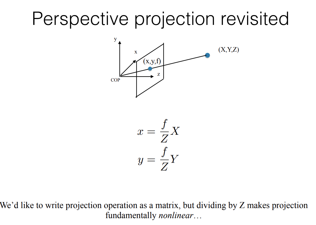
Now, the above equation can be written in matrix form, but we’ll form one artifact in this conversion i.e. lambda
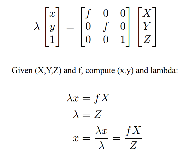
It’s clear that we can find this lambda as shown. However, why do we even need this?
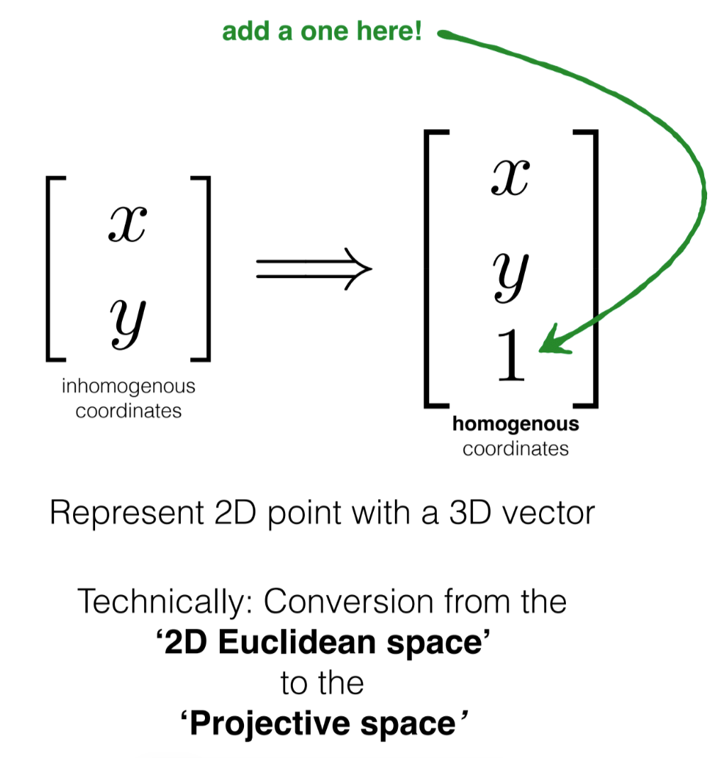
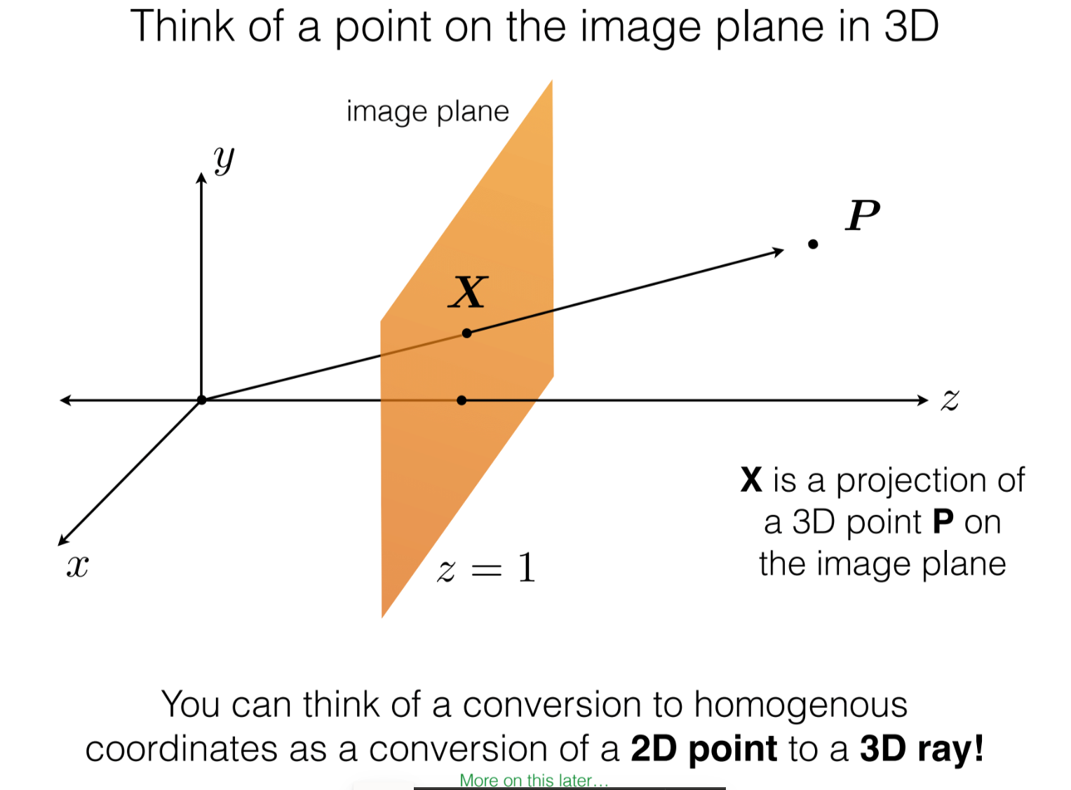
Ans. We want to represent the coordinates in homogenous coordinates
Camera Matrices
Generic Representation
Now, let’s add another constraint on this equation. Suppose we rotate our 3D point in space or we rotate the camera itself by a certain angle. In the world of robotics we call such transforms as a rotation matrix.
To get a good grasp of rotation matrices, I highly recommend some linear algebra brush-up using 3B1B (3 Blue 1 Brown). Specifically (watch 8th minute of this video) The rotation shown in the above video in the 8th minute is a rotation matrix in 2D.
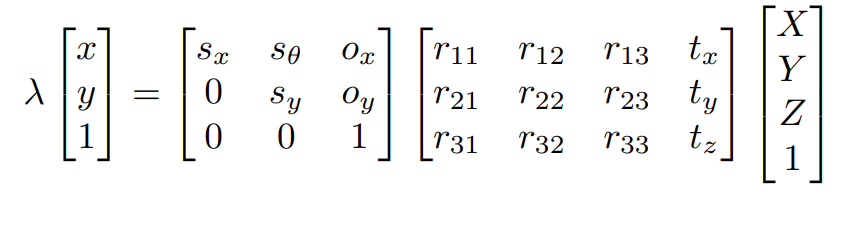
Now, adding a 3D translation (just 3 numbers which add to the x,y,z component of a 3D vector) along with a 3D rotation we get the basic projection equation
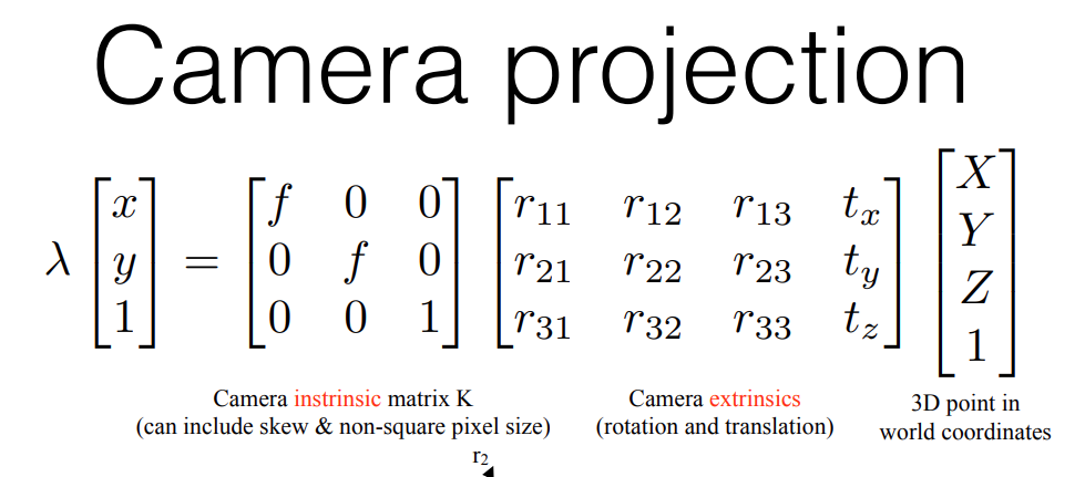
Where the two matrices are called the camera intrinsics (captures focal lengths) and the camera extrinsics (capturing rotation and translation)
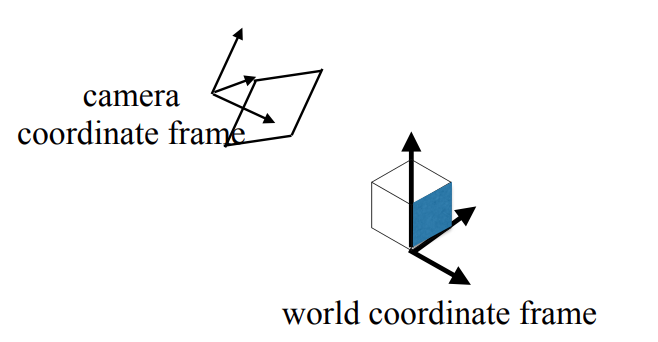
This rotation (r-matrix) can also be visualized as fixing a world coordinate frame onto some plane in the 3D world (think of a it as a flat table top) and then thinking how our camera is rotated w.r.t that frame:
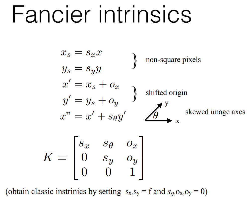
Now, most cameras also distort images due to lens optics or other properties inherent in building the camera itself. These are captured as shown below:
Now, adding these intrinsic and extrinsic factors, we get:
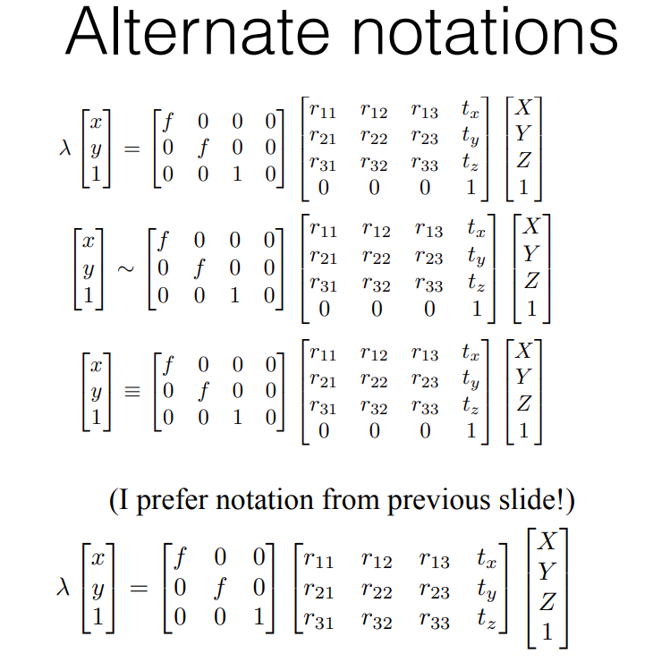
Alternate notation of camera matrices
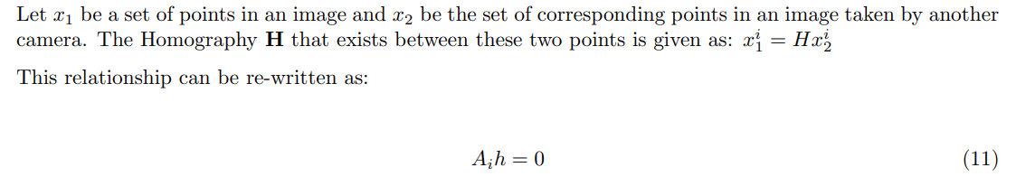
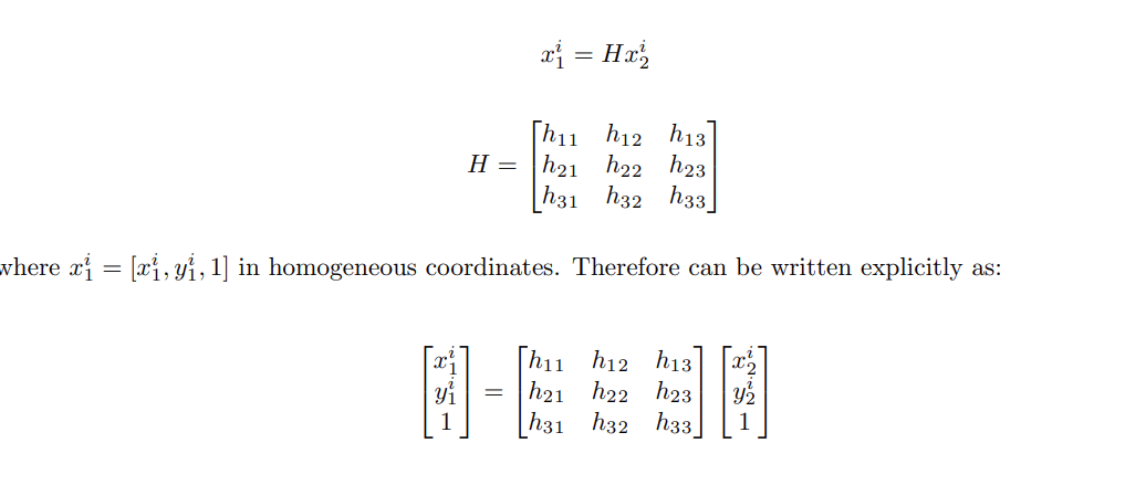
The Homography Situation
Single View
Now, if we focus on only planes (table top and human holding camera situation):
We can make certain simplifying assumptions. This is primarily that the 3D point we’re looking at has constant depth in it’s immediate neighbourhood. Using this we simplify our equations to:
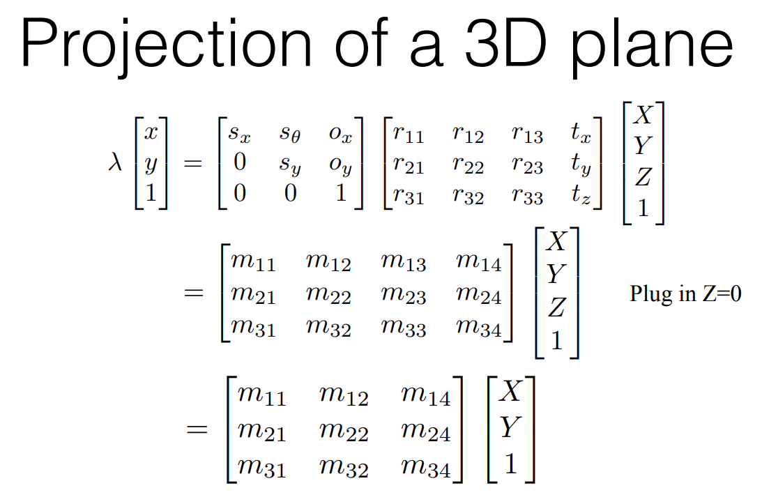
This 3x3 m-matrix now represents the mapping of 3D points on a plane to 2D point in an image
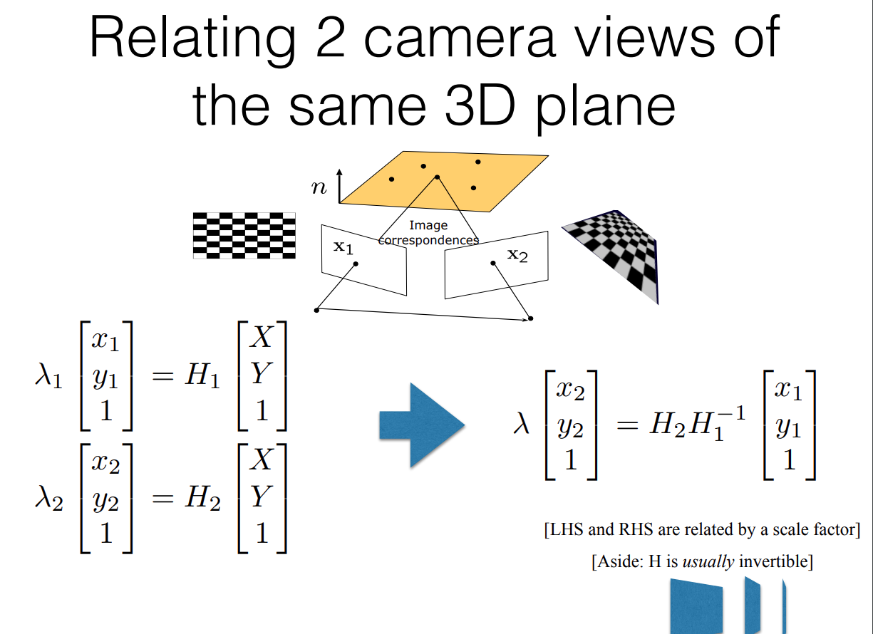
Multiple Views
Now, by simple extension of the above logic we can derive the following:
- We have just 1 plane in the 3D world
- We have two cameras looking at this plane
- Each camera has it’s own 3x3 m-matrix which maps 3D plane points onto 2D image frame
- Therefore if two cameras can see the same 3D point, we can find a mapping between the two cameras
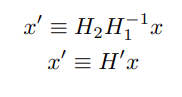
- This mapping between the two cameras is given by a new 3x3 matrix called the homography matrix
Limitations of Planar Homography
-
When the scene is very far away from the camera, all objects can be said to have the same depth. This is because the relative depth distances between foreground and background will be negligible in comparison to the average scene depth. Therefore, in such cases all objects in scene can be said to lie on a plane and as proved above, can be captured by two cameras related by a homography matrix.
-
For nearby scenes where the variation in scene depth is more apparent, a homography mapping works well only under pure rotation.
Implementation of Homography Estimation
The Pipeline
The main application of homography transforms is to find how some reference template has been warped due to movement of the camera. This is seem below as:
The applications of this are:
- image stitching (think of two images from two views as a warped version of view 0)
- augmented reality (projecting some images onto a fixed/known plane in the real world)
To perform any of the above cool applications, we first need to compute the homography between any two views. The pipeline for this would be:
- Have one reference view and another view with the camera having moved slightly
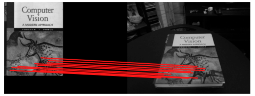
- Detect some keypoints (interest points like corners/edges) in each image
- Describe these keypoints in some way (maybe capture the histogram of pixel intensities in a small patch around the keypoint)
- Match the keypoints in one image to another using the keypoint descriptions
- Use the spatial information of these matched keypoints (i.e. the x,y coordinates of each of these keypoints) to find the Homography matrix
- **Apply the homography matrix as a transformation on one of the images **to warp and match the images
Let’s go deeper into the each of the above steps:
Keypoint Detection
- There are several methods to find keypoints in an image. Usually these keypoints are corners since other features like edges may warp or curve due to distortion and may be difficult to trace.
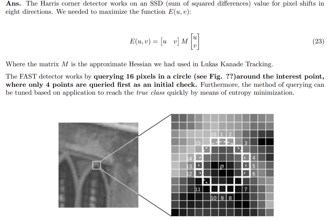
- The common methods are Harris Corner Detector, polygon fitting, FAST detectors etc.
- Here we use the FAST detector
Keypoint Descriptors
Common descriptors include BRIEF, ORB, SIFT etc. Here we’ve used the BRIEF descriptor
The BRIEF descriptor works by creating a binary feature vector of a patch from random (x,y) point pairs. This randomness in generating point pairs ensures changes in pixel intensities are captuerd in multiple directions thereby being sensitive to a large variety of edges or corners. The BRIEF descriptor also compares these binary strings using hamming distance further reduces compute time.
Due to this computational cost of calculating histograms for each filter bank it would not make sense to use filterbanks instead of BRIEF.
Further, just filterbanks cannot encode patch descriptions, i.e. without any form of histograms (like SIFT), the filterbanks themselves cannot be used instead of BRIEF.
The implementation of keypoint detection, description and matching are shown below:
import numpy as np
import cv2
import skimage.color
from helper import briefMatch
from helper import computeBrief
from helper import corner_detection

# Q2.1.4

def matchPics(I1, I2, opts):
        """
        Match features across images

        Input
        -----
        I1, I2: Source images
        opts: Command line args

        Returns
        -------
        matches: List of indices of matched features across I1, I2 [p x 2]
        locs1, locs2: Pixel coordinates of matches [N x 2]
        """
        print("computing image matches")
        ratio = opts.ratio  #'ratio for BRIEF feature descriptor'
        sigma = opts.sigma  #'threshold for corner detection using FAST feature detector'


        # Convert Images to GrayScale
        I1 = skimage.color.rgb2gray(I1)
        I2 = skimage.color.rgb2gray(I2)

        # Detect Features in Both Images
        # locs1 is just the detected corners of I1
        locs1 = corner_detection(I1, sigma)
        locs2 = corner_detection(I2, sigma)

        # Obtain descriptors for the computed feature locations
        # We use the breif descriptor to give the patch descriptions (patch of pixel width = 9)
        # for the corners(keypoints) which we obtained from corner_description

        # desc is the binary string (len(string)=256 and 256bits)
        # which serves as the feature descriptor
        desc1, locs1 = computeBrief(I1, locs1)
        desc2, locs2 = computeBrief(I2, locs2)

        # Match features using the descriptors
        matches = briefMatch(desc1, desc2, ratio)
        print(f'Computed {matches.shape[0]} matches successfully')

        return matches, locs1, locs2

def briefMatch(desc1,desc2,ratio):

    matches = skimage.feature.match_descriptors(desc1,desc2,'hamming',cross_check=True,max_ratio=ratio)
    return matches
Calculating the Homography Matrix
Let’s say we have two images: image1 and image2
To Derive the A matrix we undergo the following steps:
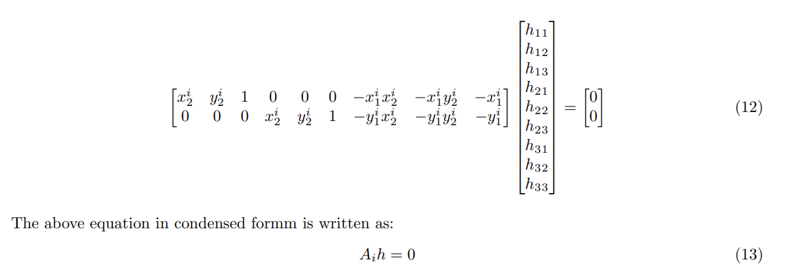
- Where h is found by taking the SVD of A and choosing the eigen vector (with least eigen value) which forms the null space of A.
- We will also normalize the correspondence points to better numerical stability of direct linear transform (DLT) estimation. Refer Normalization Document to get a better understanding of the normalization steps used below
- Remember, null-space of a vector is the transformation (i.e. transformation matrix) which squeezed the vector onto a point (i.e. it reduces dimensions to zero).
- In this case x is the vector and we find the corresponding transformation matrix which forms it’s null-space. This matrix then becomes our homography matrix
- For a better understanding of SVD, refer to This Document
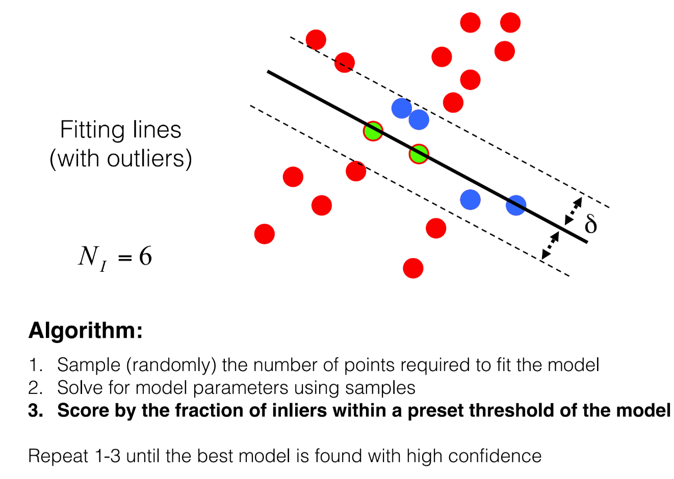
(Bonus) RANSAC: Rejecting outliers during our homography calculation
Implementation of above steps
import numpy as np
import cv2
import skimage.io
import skimage.color
from planarH import *
from opts import get_opts
from matchPics import matchPics
from helper import briefMatch

def warpImage(opts):
    """
    Warp template image based on homography transform
    Args:
        opts: user inputs
    """
    image1 = cv2.imread('../data/cv_cover.jpg')
    image2 = cv2.imread('../data/cv_desk.png')
    template_img = cv2.imread('../data/hp_cover.jpg')

    # make sure harry_potter image is same size as CV book
    x,y,z = image1.shape
    template_img = cv2.resize(template_img, (y,x))

    matches, locs1, locs2 = matchPics(image1, image2, opts)

    # invert the columns of locs1 and locs2
    locs1[:, [1, 0]] = locs1[:, [0, 1]]
    locs2[:, [1, 0]] = locs2[:, [0, 1]]

    matched_points = create_matched_points(matches, locs1, locs2)
    h, inlier = computeH_ransac(matched_points[:,0:2], matched_points[:,2:], opts)

    print("homography matrix is \n", h)

    # compositeH(h, source, destination)
    composite_img = compositeH(h, template_img, image2)

    # Display images
    cv2.imshow("Composite Image :)", composite_img)
    cv2.waitKey()

if __name__ == "__main__":

    opts = get_opts()
    warpImage(opts)
RANSAC and Construction of Composite Image
from copy import deepcopy
from dataclasses import replace
from platform import python_branch
import numpy as np
import cv2
import matplotlib.pyplot as plt
import skimage.color
import math
import random
from scipy import ndimage
from scipy.spatial import distance
from matchPics import matchPics
from helper import plotMatches
from opts import get_opts
from tqdm import tqdm


def computeH(x1, x2):
    """
    Computes the homography based on
    matching points in both images

    Args:
        x1: keypoints in image 1
        x2: keypoints in image 2

    Returns:
        H2to1: the homography matrix
    """

    # Define a dummy H matrix
    A_build = []

    # Define the A matrix for (Ah = 0) (A matrix size = N*2 x 9)
    for i in range(x1.shape[0]):
        row_1 = np.array([ x2[i,0], x2[i,1], 1, 0, 0, 0, -x1[i,0]*x2[i,0], -x1[i,0]*x2[i,1], -x1[i,0] ])
        row_2 = np.array([ 0, 0, 0, x2[i,0], x2[i,1], 1, -x1[i,1]*x2[i,0], -x1[i,1]*x2[i,1], -x1[i,1] ])
        A_build.append(row_1)
        A_build.append(row_2)

    A = np.stack(A_build, axis=0)

    # Do the least squares minimization to get the homography matrix
    # this is done as eigenvector coresponding to smallest eigen value of A`A = H matrix
    u, s, v = np.linalg.svd(np.matmul(A.T, A))

    # here the linalg.svd gives v_transpose
    # but we need just V therefore we again transpose
    H2to1 = np.reshape(v.T[:,-1], (3,3))
    return H2to1


def computeH_norm(x1, x2):
    #Q2.2.2
    """
    Compute the normalized coordinates
    and also the homography matrix using computeH

    Args:
        x1 (Mx2): the matched locations of corners in img1
        x2 (Mx2): the matched locations of corners in img2

    Returns:
        H2to1: Hmography matrix after denormalization
    """
    # Q2.2.2
    # Compute the centroid of the points
    centroid_img_1 = np.sum(x1, axis=0)/x1.shape[0]
    centroid_img_2 = np.sum(x2, axis=0)/x2.shape[0]

    # print(f'centroid of img1 is {centroid_img_1} \n centroid of img2 is {centroid_img_2}')

    # Shift the origin of the points to the centroid
    # let origin for img1 be centroid_img_1 and similarly for img2
    #? Now translate every point such that centroid is at [0,0]
    moved_x1 = x1 - centroid_img_1
    moved_x2 = x2 - centroid_img_2

    current_max_dist_img1 = np.max(np.linalg.norm(moved_x1),axis=0)
    current_max_dist_img2 = np.max(np.linalg.norm(moved_x2),axis=0)


    # moved and scaled image 1 points
    scale1 = np.sqrt(2) / (current_max_dist_img1)
    scale2 = np.sqrt(2) / (current_max_dist_img2)
    moved_scaled_x1 = moved_x1 * scale1
    moved_scaled_x2 = moved_x2 * scale2

    # Similarity transform 1
    #? We construct the transformation matrix to be 3x3 as it has to be same shape of Homography
    t1 = np.diag([scale1, scale1, 1])
    t1[0:2,2] = -scale1*centroid_img_1

    # Similarity transform 2
    t2 = np.diag([scale2, scale2, 1])
    t2[0:2,2] = -scale2*centroid_img_2

    # Compute homography
    H = computeH(moved_scaled_x1, moved_scaled_x2)

    # Denormalization
    H2to1 = np.matmul(np.linalg.inv(t1), np.matmul(H, t2))

    return H2to1

def create_matched_points(matches, locs1, locs2):
    """
    Match the corners in img1 and img2 according to the BRIEF matched points

    Args:
        matches (Mx2): Vector containing the index of locs1 and locs2 which matches
        locs1 (Nx2): Vector containing corner positions for img1
        locs2 (Nx2):  Vector containing corner positions for img2

    Returns:
        _type_: _description_
    """
    matched_pts = []
    for i in range(matches.shape[0]):
        matched_pts.append(np.array([locs1[matches[i,0],0],
                                              locs1[matches[i,0],1],
                                              locs2[matches[i,1],0],
                                              locs2[matches[i,1],1]]))

    # remove the first dummy value and return
    matched_points = np.stack(matched_pts, axis=0)
    return matched_points

def computeH_ransac(locs1, locs2, opts):
    """
    Every iteration we init a Homography matrix using 4 corresponding
    points and calculate number of inliers. Finally use the Homography
    matrix which had max number of inliers (and these inliers as well)
    to find the final Homography matrix
    Args:
        locs1: location of matched points in image1
        locs2: location of matched points in image2
        opts: user inputs used for distance tolerance in ransac

    Returns:
        bestH2to1     : The homography matrix with max number of inliers
        final_inliers : Final list of inliers considered for homography
    """
    #Q2.2.3
    #Compute the best fitting homography given a list of matching points

    max_iters = opts.max_iters  # the number of iterations to run RANSAC for
    inlier_tol = opts.inlier_tol # the tolerance value for considering a point to be an inlier

    # define size of both locs1 and locs2
    num_rows = locs1.shape[0]

    # define a container for keeping track of inlier counts
    final_inlier_count = 0
    final_distance_error = 10000

    #? Create a boolean vector of length N where 1 = inlier and 0 = outlier
    print("Computing RANSAC")
    for i in range(max_iters):
        test_locs1 = deepcopy(locs1)
        test_locs2 = deepcopy(locs2)
        # chose a random sample of 4 points to find H
        rand_index = []

        rand_index = random.sample(range(int(locs1.shape[0])),k=4)

        rand_points_1 = []
        rand_points_2 = []

        for j in rand_index:
            rand_points_1.append(locs1[j,:])
            rand_points_2.append(locs2[j,:])

        test_locs1 = np.delete(test_locs1, rand_index, axis=0)
        test_locs2 = np.delete(test_locs2, rand_index, axis=0)

        correspondence_points_1 = np.vstack(rand_points_1)
        correspondence_points_2 = np.vstack(rand_points_2)

        ref_H = computeH_norm(correspondence_points_1, correspondence_points_2)
        inliers, inlier_count, distance_error, error_state = compute_inliers(ref_H,
                                                                            test_locs1,
                                                                            test_locs2,
                                                                            inlier_tol)

        if error_state == 1:
            continue

        if (inlier_count > final_inlier_count) and (distance_error < final_distance_error):
            final_inlier_count = inlier_count
            final_inliers = inliers
            final_corresp_points_1 = correspondence_points_1
            final_corresp_points_2 = correspondence_points_2
            final_distance_error = distance_error
            final_test_locs1 = test_locs1
            final_test_locs2 = test_locs2

    if final_distance_error != 10000:
        # print("original point count is", locs1.shape[0])
        # print("final inlier count is", final_inlier_count)
        # print("final inlier's cumulative distance error is", final_distance_error)

        delete_indexes = np.where(final_inliers==0)
        final_locs_1 = np.delete(final_test_locs1, delete_indexes, axis=0)
        final_locs_2 = np.delete(final_test_locs2, delete_indexes, axis=0)

        final_locs_1 = np.vstack((final_locs_1, final_corresp_points_1))
        final_locs_2 = np.vstack((final_locs_2, final_corresp_points_2))

        bestH2to1 = computeH_norm(final_locs_1, final_locs_2)
        return bestH2to1, final_inliers

    else:
        bestH2to1 = computeH_norm(correspondence_points_1, correspondence_points_2)
        return bestH2to1, 0

def compute_inliers(h, x1, x2, tol):
    """
    Compute the number of inliers for a given
    homography matrix
    Args:
        h: Homography matrix
        x1 : matched points in image 1
        x2 : matched points in image 2
        tol: tolerance value to check for inliers

    Returns:
        inliers         : indexes of x1 or x2 which are inliers
        inlier_count    : number of total inliers
        dist_error_sum  : Cumulative sum of errors in reprojection error calc
        flag            : flag to indicate if H was invertible or not
    """
    # take H inv to map points in x1 to x2
    try:
        H = np.linalg.inv(h)
    except:
        return [1,1,1], 1, 1, 1

    x2_extd = np.append(x2, np.ones((x2.shape[0],1)), axis=1)
    x1_extd = (np.append(x1, np.ones((x1.shape[0],1)), axis=1))
    x2_est = np.zeros((x2_extd.shape), dtype=x2_extd.dtype)

    for i in range(x1.shape[0]):
        x2_est[i,:] = H @ x1_extd[i,:]

    x2_est = x2_est/np.expand_dims(x2_est[:,2], axis=1)
    dist_error = np.linalg.norm((x2_extd-x2_est),axis=1)

    # print("dist error is", dist_error)
    inliers = np.where((dist_error < tol), 1, 0)
    inlier_count = np.count_nonzero(inliers == 1)

    return inliers, inlier_count, np.sum(dist_error), 0


def compositeH(H2to1, template, img):
    """
    Create a composite image after warping the template image on top
    of the image using the homography

    Args:
        H2to1 : Existing(already found) homography matrix
        template: Harry Potter (template image)
        img: Base image onto which we overlay Harry Potter image

    Returns:
        composite_img: Base image with overlayed Harry Potter cover
    """
    output_shape = (img.shape[1],img.shape[0])
    # destination_img = img
    # source_img = template
    h = np.linalg.inv(H2to1)

    # Create mask of same size as template
    mask = np.ones((template.shape[0], template.shape[1]))*255
    mask = np.stack((mask, mask, mask), axis=2)

    # Warp mask by appropriate homography
    warped_mask = cv2.warpPerspective(mask, h, output_shape)

    # Warp template by appropriate homography
    warped_template = cv2.warpPerspective(template, h, output_shape)

    # Use mask to combine the warped template and the image
    composite_img = np.where(warped_mask, warped_template, img)

    return composite_img


def panorama_composite(H2to1, template, img):
    """
    Stitch two images together to form a panorama

    Args:
        H2to1: Homography Matrix
        template: The pano_right image
        img: The pano_left image

    Returns:
        composite_img: Stitched image (panorama)
    """
    output_shape = (img.shape[1]+240,img.shape[0]+240)
    # destination_img = img
    # source_img = template
    h = H2to1

    img_padded = np.zeros((img.shape[0]+240,img.shape[1]+240,3), dtype=img.dtype)
    img_padded[0:img.shape[0], 0:img.shape[1], :] = img[:,:,:]

    # Create mask of same size as template
    mask = np.ones((template.shape[0], template.shape[1]))*255
    mask = np.stack((mask, mask, mask), axis=2)

    # Warp mask by appropriate homography
    warped_mask = cv2.warpPerspective(mask, h, output_shape)

    # Warp template by appropriate homography
    cv2.imshow("template image", template)
    cv2.waitKey()
    cv2.imshow("destination image", img)
    cv2.waitKey()
    warped_template = cv2.warpPerspective(template, h, output_shape)

    cv2.imshow("warped template", warped_template)
    cv2.waitKey()

    # Use mask to combine the warped template and the image
    composite_img = np.where(warped_mask, warped_template, img_padded)

    return composite_img
Applying Homography Estimation in the Real World
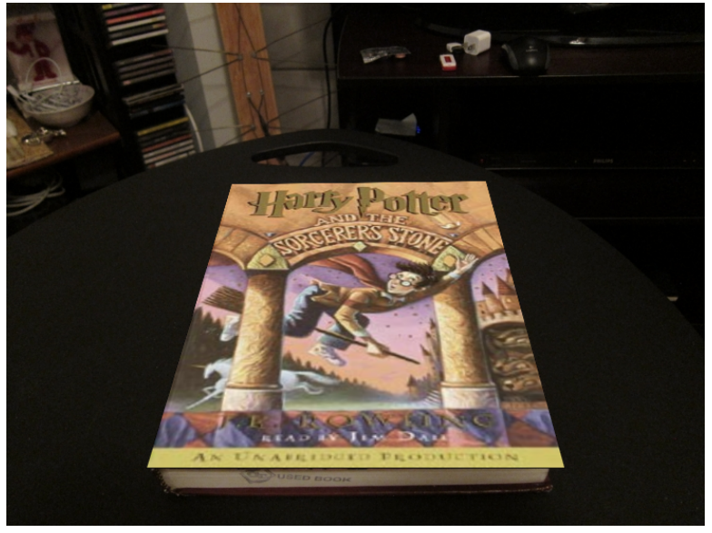
Basic cool applications
If we know how a template matches to a warped image, such as:
We can then use this homography matrix to map any plane (here a different book cover) onto our destination image
AR Video
Here we use the same book-cover homography mapping but onto a sequence of frames of a video
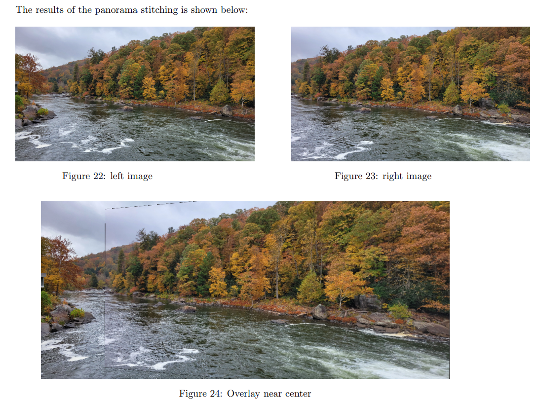
Panorama Stitching
During my visit to Ohiopyle, I took few pictures of the river. Let’s back to the fact that homography works well for far away scenes, where the large distance from camera to landscape makes the relative distances of objects in the landscape negligible. In such cases even small translations of the camera have a small effect on the landscape itself.
However, since the scene at ohiopyle was not too far away, any translation would yield a bad homography matrix and cause shoddy stitching. Therefore I tried to mitigate this by only rotating about my hip (to ensure no translational movement) while taking the two views.
The results of the stitching are shown below:
Acknowledgement and References
A lot of images are taken from the lecture slides during my computer vision class at CMU. These were taught by Prof. Kris Kitani and Prof. Deva Ramanan
These slides are publicly available (slides)
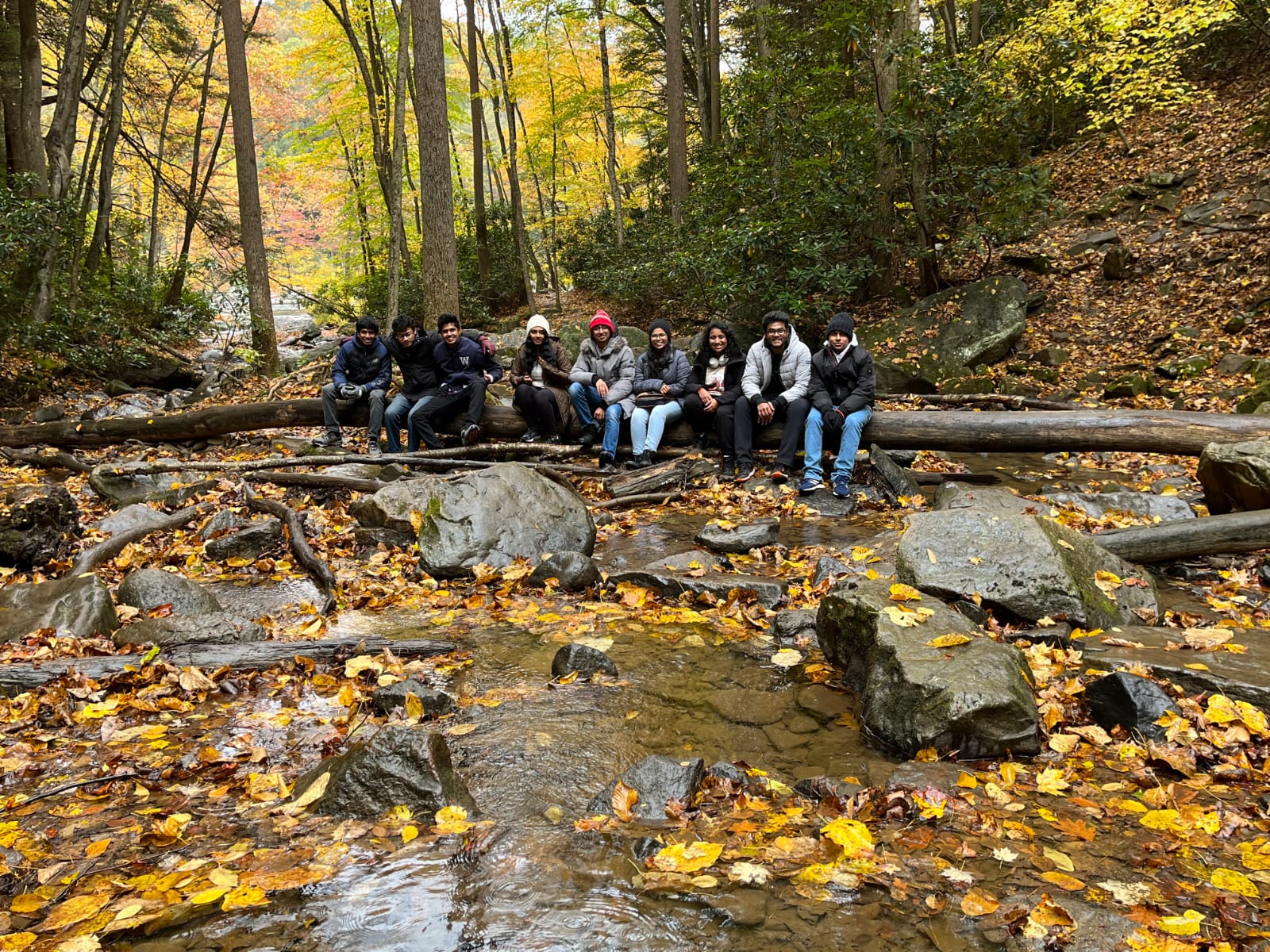
My Ohiopyle trip
Helper Functions
The helper function in this framework is shown below:
import numpy as np
import cv2
import scipy.io as sio
from matplotlib import pyplot as plt
import skimage.feature

PATCHWIDTH = 9

def briefMatch(desc1,desc2,ratio):

    matches = skimage.feature.match_descriptors(desc1,desc2,'hamming',cross_check=True,max_ratio=ratio)
    return matches


def plotMatches(im1,im2,matches,locs1,locs2):

    fig, ax = plt.subplots(nrows=1, ncols=1)
    im1 = cv2.cvtColor(im1, cv2.COLOR_BGR2GRAY)
    im2 = cv2.cvtColor(im2, cv2.COLOR_BGR2GRAY)
    plt.axis('off')
    skimage.feature.plot_matches(ax,im1,im2,locs1,locs2,matches,matches_color='r',only_matches=True)
    plt.show()
    return


def makeTestPattern(patchWidth, nbits):

    np.random.seed(0)
    compareX = patchWidth*patchWidth * np.random.random((nbits,1))
    compareX = np.floor(compareX).astype(int)
    np.random.seed(1)
    compareY = patchWidth*patchWidth * np.random.random((nbits,1))
    compareY = np.floor(compareY).astype(int)

    return (compareX, compareY)


def computePixel(img, idx1, idx2, width, center):

    halfWidth = width // 2
    col1 = idx1 % width - halfWidth
    row1 = idx1 // width - halfWidth
    col2 = idx2 % width - halfWidth
    row2 = idx2 // width - halfWidth
    return 1 if img[int(center[0]+row1)][int(center[1]+col1)] < img[int(center[0]+row2)][int(center[1]+col2)] else 0


def computeBrief(img, locs):

    patchWidth = 9
    nbits = 256
    compareX, compareY = makeTestPattern(patchWidth,nbits)
    m, n = img.shape

    halfWidth = patchWidth//2

    locs = np.array(list(filter(lambda x: halfWidth <= x[0] < m-halfWidth and halfWidth <= x[1] < n-halfWidth, locs)))
    desc = np.array([list(map(lambda x: computePixel(img, x[0], x[1], patchWidth, c), zip(compareX, compareY))) for c in locs])

    return desc, locs


def corner_detection(img, sigma):

    # fast method
    result_img = skimage.feature.corner_fast(img, n=PATCHWIDTH, threshold=sigma)
    locs = skimage.feature.corner_peaks(result_img, min_distance=1)
    return locs


def loadVid(path):

    # Create a VideoCapture object and read from input file
    # If the input is the camera, pass 0 instead of the video file name

    cap = cv2.VideoCapture(path)

    # Append frames to list
    frames = []

    # Check if camera opened successfully
    if cap.isOpened()== False:
        print("Error opening video stream or file")

    # Read until video is completed
    while(cap.isOpened()):

        # Capture frame-by-frame
        ret, frame = cap.read()

        if ret:
            #Store the resulting frame
            frames.append(frame)
        else:
            break

    # When everything done, release the video capture object
    cap.release()
    frames = np.stack(frames)

    return frames